The animation show the Trimmed Grassmann Average (TGA) algorithm on synthetic data (orange circles). The algorithm is initialized roughly orthogonal to the correct component. In each iteration, all observations are given a sign to be as similar as possible to the current component estimate. The component (blue line) is then updated as the trimmed mean of the re-signed data (green circles). This is repeated until convergence.
As the collection of large datasets becomes increasingly automated, the occurrence of outliers will increase -- big data implies big outliers. As a scalable approach to robust PCA we propose to compute the average subspace spanned by the data; this can then be made robust by computing robust averages.
This page provides source code and video material for the paper Grassmann Averages for Scalable Robust PCA.
2 Dept. of Computer Science, University of Copenhagen

We provide implementations for the Grassmann Average, the Trimmed Grassmann Average, and the Grassmann Median. We the simplest is the Matlab implementation used in the CVPR 2014 paper, but we also provide a faster C++ implementation, which can be used either directly from C++ or through a Matlab wrapper interface. The code is available for download below. Any feedback is much appreciated and can be send to Søren Hauberg.
C++ Implementation
A highly parallel C++ implementation of the Grassmann averages are available at the Tübingen OwnCloud. This includes both a C++ library and a Matlab interface. This is the recommended implementation of the algorithms.
Matlab Implementation
The simplest implementation is done in pure Matlab, with a C++ implementation of trimmed averages. This implementation was used for the CVPR 2014 paper. With the release of the pure C++ implementation, this code is mostly useful for understanding the basic algorithms.
Example Code
As a simple example, we will first generate samples from a random Gaussian distribution, and then estimate its leading component.
  D = 2; % we consider a two-dimensional problem
  N = 100; % we will generate 100 observations

  %% Generate a random Covariance matrix
  tmp = randn(D);
  Sigma = tmp.' * tmp;

  %% Sample from the corresponding Gaussian
  X = mvnrnd(zeros(D, 1), Sigma, N);

  %% Estimate the leading component
  comp = grassmann_average(X, 1); % the second input is the number of component to estimate

  %% Plot the results
  plot(X(:, 1), X(:, 2), 'ko', 'markerfacecolor', [255,153,51]./255);
  axis equal
  hold on
  plot(3*[-comp(1), comp(1)], 3*[-comp(2), comp(2)], 'k', 'linewidth', 2)
  hold off
  axis off
This produces a plot like the figure below. 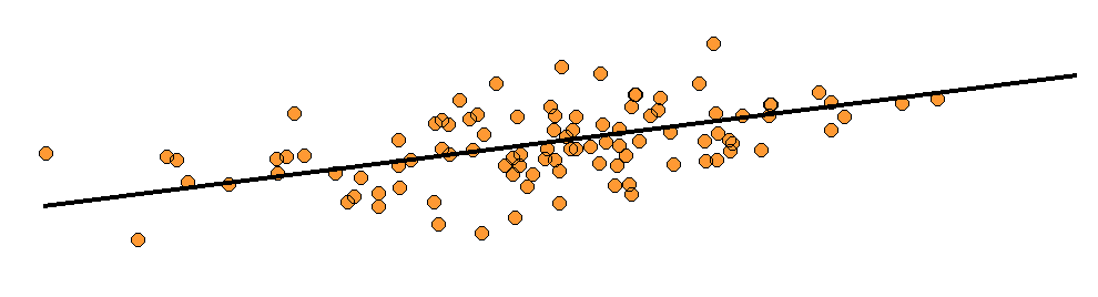
Download
The initial version of the Matlab code is now available: grassmann_averages-0.3.zip. For questions or comments please contact Søren Hauberg.
Spotlight
The video spotlight for CVPR 2014 provides a brief overview of the contributions of the Grassmann Average.
Tutorial
The main idea in the Grassmann Average paper is sketched in the video below.
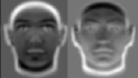
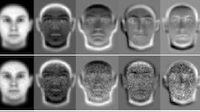
Results
Some of the results in the CVPR 2014 paper are shown in the video below.